Pranav Rajan’s Blog - FastAI Lesson 6: Random Forests

Acknowledgements

All of this code was written by Jeremy Howard and the FastAI team. I modified it slightly to include my own print statements, comments and additional helper functions based on Jeremy’s code. This is the source for the original code How random forests really work, First Steps: Road to the Top, Part 1 and Small models: Road to the Top, Part 2.

Summary

In this lesson, Jeremy goes over Random Forests, Decision Trees, Binary Splits, Bagging and Gradient Boosting. Towards the middle half of the lesson, Jeremy starts a deep dive of his process in achieving the top scores for the Paddy Doctor: Paddy Disease Classification challenge.

Jeremy Howard’s Advice

In datasets with many columns, creating a feature importance plot early is helpful in finding which columns are worth studying more closely
Complex models are not always better
Simple models will have trouble providing adequate accuracy for more complex tasks such as recommendation systems, NLP, computer vision, or multivariate time series
Random forests are not sensitive to issues like normalization, interactions, non-linear transformations which make them easy to work with and hard to mess up

Load Data and Libraries

# import libraries and files

# required libraries + packages for any ml/data science project
import numpy as np
import pandas as pd
import matplotlib.pyplot as plt
import torch

# fastai library contains all the packages above and wraps them in the fastai library
!pip install -Uqq fastai

# kaggle API package install
!pip install kaggle

# install TIMM
!pip install timm

Requirement already satisfied: kaggle in /usr/local/lib/python3.10/dist-packages (1.5.16)
Requirement already satisfied: six>=1.10 in /usr/local/lib/python3.10/dist-packages (from kaggle) (1.16.0)
Requirement already satisfied: certifi in /usr/local/lib/python3.10/dist-packages (from kaggle) (2023.11.17)
Requirement already satisfied: python-dateutil in /usr/local/lib/python3.10/dist-packages (from kaggle) (2.8.2)
Requirement already satisfied: requests in /usr/local/lib/python3.10/dist-packages (from kaggle) (2.31.0)
Requirement already satisfied: tqdm in /usr/local/lib/python3.10/dist-packages (from kaggle) (4.66.1)
Requirement already satisfied: python-slugify in /usr/local/lib/python3.10/dist-packages (from kaggle) (8.0.1)
Requirement already satisfied: urllib3 in /usr/local/lib/python3.10/dist-packages (from kaggle) (2.0.7)
Requirement already satisfied: bleach in /usr/local/lib/python3.10/dist-packages (from kaggle) (6.1.0)
Requirement already satisfied: webencodings in /usr/local/lib/python3.10/dist-packages (from bleach->kaggle) (0.5.1)
Requirement already satisfied: text-unidecode>=1.3 in /usr/local/lib/python3.10/dist-packages (from python-slugify->kaggle) (1.3)
Requirement already satisfied: charset-normalizer<4,>=2 in /usr/local/lib/python3.10/dist-packages (from requests->kaggle) (3.3.2)
Requirement already satisfied: idna<4,>=2.5 in /usr/local/lib/python3.10/dist-packages (from requests->kaggle) (3.6)
Collecting timm
  Downloading timm-0.9.12-py3-none-any.whl (2.2 MB)
     ━━━━━━━━━━━━━━━━━━━━━━━━━━━━━━━━━━━━━━━━ 2.2/2.2 MB 10.5 MB/s eta 0:00:00
Requirement already satisfied: torch>=1.7 in /usr/local/lib/python3.10/dist-packages (from timm) (2.1.0+cu121)
Requirement already satisfied: torchvision in /usr/local/lib/python3.10/dist-packages (from timm) (0.16.0+cu121)
Requirement already satisfied: pyyaml in /usr/local/lib/python3.10/dist-packages (from timm) (6.0.1)
Requirement already satisfied: huggingface-hub in /usr/local/lib/python3.10/dist-packages (from timm) (0.20.2)
Requirement already satisfied: safetensors in /usr/local/lib/python3.10/dist-packages (from timm) (0.4.1)
Requirement already satisfied: filelock in /usr/local/lib/python3.10/dist-packages (from torch>=1.7->timm) (3.13.1)
Requirement already satisfied: typing-extensions in /usr/local/lib/python3.10/dist-packages (from torch>=1.7->timm) (4.5.0)
Requirement already satisfied: sympy in /usr/local/lib/python3.10/dist-packages (from torch>=1.7->timm) (1.12)
Requirement already satisfied: networkx in /usr/local/lib/python3.10/dist-packages (from torch>=1.7->timm) (3.2.1)
Requirement already satisfied: jinja2 in /usr/local/lib/python3.10/dist-packages (from torch>=1.7->timm) (3.1.3)
Requirement already satisfied: fsspec in /usr/local/lib/python3.10/dist-packages (from torch>=1.7->timm) (2023.6.0)
Requirement already satisfied: triton==2.1.0 in /usr/local/lib/python3.10/dist-packages (from torch>=1.7->timm) (2.1.0)
Requirement already satisfied: requests in /usr/local/lib/python3.10/dist-packages (from huggingface-hub->timm) (2.31.0)
Requirement already satisfied: tqdm>=4.42.1 in /usr/local/lib/python3.10/dist-packages (from huggingface-hub->timm) (4.66.1)
Requirement already satisfied: packaging>=20.9 in /usr/local/lib/python3.10/dist-packages (from huggingface-hub->timm) (23.2)
Requirement already satisfied: numpy in /usr/local/lib/python3.10/dist-packages (from torchvision->timm) (1.23.5)
Requirement already satisfied: pillow!=8.3.*,>=5.3.0 in /usr/local/lib/python3.10/dist-packages (from torchvision->timm) (9.4.0)
Requirement already satisfied: MarkupSafe>=2.0 in /usr/local/lib/python3.10/dist-packages (from jinja2->torch>=1.7->timm) (2.1.3)
Requirement already satisfied: charset-normalizer<4,>=2 in /usr/local/lib/python3.10/dist-packages (from requests->huggingface-hub->timm) (3.3.2)
Requirement already satisfied: idna<4,>=2.5 in /usr/local/lib/python3.10/dist-packages (from requests->huggingface-hub->timm) (3.6)
Requirement already satisfied: urllib3<3,>=1.21.1 in /usr/local/lib/python3.10/dist-packages (from requests->huggingface-hub->timm) (2.0.7)
Requirement already satisfied: certifi>=2017.4.17 in /usr/local/lib/python3.10/dist-packages (from requests->huggingface-hub->timm) (2023.11.17)
Requirement already satisfied: mpmath>=0.19 in /usr/local/lib/python3.10/dist-packages (from sympy->torch>=1.7->timm) (1.3.0)
Installing collected packages: timm
Successfully installed timm-0.9.12

from fastai.imports import *
import os
from pathlib import Path
import zipfile

'''Function for loading kaggle datasets locally or on kaggle
Returns a local path to data files
- input: Kaggle API Login Credentials, Kaggle Contest Name '''
def loadData(creds, dataFile):
    # variable to check whether we're running on kaggle website or not
    iskaggle = os.environ.get('KAGGLE_KERNEL_RUN_TYPE', '')

    # path for kaggle API credentials
    cred_path = Path('~/.kaggle/kaggle.json').expanduser()

    if not cred_path.exists():
        cred_path.parent.mkdir(exist_ok=True)
        cred_path.write_text(creds)
        cred_path.chmod(0o600)

    # Download data from Kaggle to path and extract files at path location

    # local machine
    path = Path(dataFile)
    if not iskaggle and not path.exists():
        import kaggle
        kaggle.api.competition_download_cli(str(path))
        zipfile.ZipFile(f'{path}.zip').extractall(path)

    # kaggle
    if iskaggle:
        fileName = '../input/' + dataFile
        path = fileName

    return path

creds = ''
dataFile = 'titanic'
path = loadData(creds, dataFile)

Downloading titanic.zip to /content

100%|██████████| 34.1k/34.1k [00:00<00:00, 38.4MB/s]

# check data files
! ls {path}

gender_submission.csv  test.csv  train.csv

# set up default settings
import warnings, logging, torch
warnings.simplefilter('ignore')
logging.disable(logging.WARNING)
np.set_printoptions(linewidth=130)

# load data files and find modes of categories
df = pd.read_csv(path/'train.csv')
tst_df = pd.read_csv(path/'test.csv')
modes = df.mode().iloc[0]

Exploratory Data Analysis

Exploratory Data Analysis: Data Preprocessing

# Standardize data types for modeling with random forests
def proc_data(df):
    df['Fare'] = df.Fare.fillna(0)
    df.fillna(modes, inplace=True)
    df['LogFare'] = np.log1p(df['Fare'])
    df['Embarked'] = pd.Categorical(df.Embarked)
    df['Sex'] = pd.Categorical(df.Sex)

proc_data(df)
proc_data(tst_df)

Exploratory Data Analysis: Data Exploration

# categorical variables
cats=["Sex","Embarked"]

# continuous variables
conts=['Age', 'SibSp', 'Parch', 'LogFare',"Pclass"]

# dependent variable (the thing we're trying to determine)
dep="Survived"

df.Sex.head()

0      male
1    female
2    female
3    female
4      male
Name: Sex, dtype: category
Categories (2, object): ['female', 'male']

df.Sex.cat.codes.head()

0    1
1    0
2    0
3    0
4    1
dtype: int8

Binary Split

Random forests are made up of decision trees
Decision trees are made up of binary splits
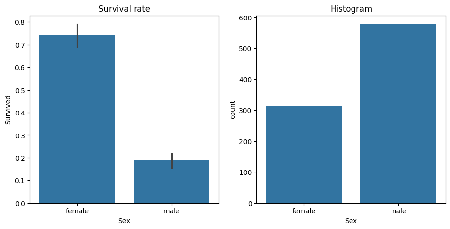
Binary Split: all rows placed into one of two groups based on whether they are above or below some threshold of some column. Example: Threshold = 0.5 and column Sex (0 represents females, 1 represents males)

import seaborn as sns

fig,axs = plt.subplots(1,2, figsize=(11,5))
sns.barplot(data=df, y=dep, x="Sex", ax=axs[0]).set(title="Survival rate")
sns.countplot(data=df, x="Sex", ax=axs[1]).set(title="Histogram")

[Text(0.5, 1.0, 'Histogram')]

Simple Model - Categorical Variable Split: All females survive and no males do

# split training data into training and validation data
# - 25% validation, 75% training

from numpy import random
from sklearn.model_selection import train_test_split

random.seed(42)
trn_df,val_df = train_test_split(df, test_size=0.25)
trn_df[cats] = trn_df[cats].apply(lambda x: x.cat.codes)
val_df[cats] = val_df[cats].apply(lambda x: x.cat.codes)

# create independent and dependent variables
def xs_y(df):
    xs = df[cats + conts].copy()
    return xs,df[dep] if dep in df else None

trn_xs,trn_y = xs_y(trn_df)
val_xs,val_y = xs_y(val_df)

# predictions for simple model -> female is coded as 0
preds = val_xs.Sex==0

# metrics (loss function) - Mean Absolute Error
from sklearn.metrics import mean_absolute_error
mean_absolute_error(val_y, preds)

0.21524663677130046

Simple Model - Continuous Variable Split: Log Fare

# - 0 -> did not survive
# - 1 -> survived
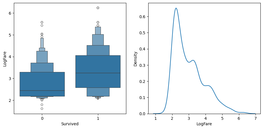
# - boxen plot shows the average logfare for passengers that didn't survive is around 2.5
# and for those who did survive it was around 3.2

df_fare = trn_df[trn_df.LogFare>0]
fig,axs = plt.subplots(1,2, figsize=(11,5))
sns.boxenplot(data=df_fare, x=dep, y="LogFare", ax=axs[0])
sns.kdeplot(data=df_fare, x="LogFare", ax=axs[1])

<Axes: xlabel='LogFare', ylabel='Density'>

# predictions
# - based on the plots, data is showing that people who paid more for tickets were more likely to get put on lifeboat

# test theory
preds = val_xs.LogFare > 2.7

# less accurate than the previous model
mean_absolute_error(val_y, preds)

0.336322869955157

Metric: Score Function

Score calculates a measure of impurity, how much the binary split creates two groups where the rows in a group are each similar to each other, or dissimilar
The similarity of rows inside a group can be measured by taking the standard deviation of the dependent variable
The higher the SDthn the rows are more different to each other
Multiply the SD by the number of rows since a bigger group has more impact than a smaller group

# - need a function to determine how good model is based on different splits
# - need a way to try more columns and splits
# - instead of MAE use a function that calculates a measure of impurity ->
# how much the binary split creates two groups where the rows in a group are each similar to each other or dissimilar
from ipywidgets import interact

def _side_score(side, y):
    tot = side.sum()
    if tot <= 1:
      return 0
    return y[side].std() * tot

# - calculate the score for a split by adding up the scores for the left hand side and right hand side
def score(col, y, split):
    lhs = col<= split
    return (_side_score(lhs,y) + _side_score(~lhs,y)) / len(y)

# compute score for a particular variable (categorical, continuous)
def iscore(nm, split):
    col = trn_xs[nm]
    return score(col, trn_y, split)

# find the best split threshold for a particular variable (categorical, continuous)
# function for finding best split
def min_col(df, nm):
    col,y = df[nm],df[dep]
    unq = col.dropna().unique()
    scores = np.array([score(col, y, o) for o in unq if not np.isnan(o)])
    idx = scores.argmin()
    return unq[idx],scores[idx]

# impurity score for Sex Split
score(trn_xs["Sex"], trn_y, 0.5)

0.40787530982063946

# impurity score for Log Fare
score(trn_xs["LogFare"], trn_y, 2.7)

0.47180873952099694

# interactive widget for finding the best threshold and split for continuous variables
interact(nm=conts, split=15.5)(iscore)

<function __main__.iscore(nm, split)>

# interactive widget for finding best threshold and split for categorical variables
interact(nm=cats, split=2)(iscore)

<function __main__.iscore(nm, split)>

# Automating Split Finding - Find Split for Age
nm = "Age"
col = trn_xs[nm]
unq = col.unique()
unq.sort()
unq

array([ 0.42,  0.67,  0.75,  0.83,  0.92,  1.  ,  2.  ,  3.  ,  4.  ,  5.  ,  6.  ,  7.  ,  8.  ,  9.  , 10.  , 11.  , 12.  ,
       13.  , 14.  , 14.5 , 15.  , 16.  , 17.  , 18.  , 19.  , 20.  , 21.  , 22.  , 23.  , 24.  , 24.5 , 25.  , 26.  , 27.  ,
       28.  , 28.5 , 29.  , 30.  , 31.  , 32.  , 32.5 , 33.  , 34.  , 34.5 , 35.  , 36.  , 36.5 , 37.  , 38.  , 39.  , 40.  ,
       40.5 , 41.  , 42.  , 43.  , 44.  , 45.  , 45.5 , 46.  , 47.  , 48.  , 49.  , 50.  , 51.  , 52.  , 53.  , 54.  , 55.  ,
       55.5 , 56.  , 57.  , 58.  , 59.  , 60.  , 61.  , 62.  , 64.  , 65.  , 70.  , 70.5 , 74.  , 80.  ])

# find index where score is the lowest
scores = np.array([score(col, trn_y, o) for o in unq if not np.isnan(o)])
unq[scores.argmin()]

# - In Age column, 6 is the optimal threshold cutoff in the training set

6.0

# test split finding function on age category
min_col(trn_df, "Age")

(6.0, 0.478316717508991)

# find best split for all variables
cols = cats + conts

{o:min_col(trn_df, o) for o in cols}

{'Sex': (0, 0.40787530982063946),
 'Embarked': (0, 0.47883342573147836),
 'Age': (6.0, 0.478316717508991),
 'SibSp': (4, 0.4783740258817434),
 'Parch': (0, 0.4805296527841601),
 'LogFare': (2.4390808375825834, 0.4620823937736597),
 'Pclass': (2, 0.46048261885806596)}

Decision Tree

Take each group (male, female) and create one more binary split for each group
Find the single best split for male, and single best split for female
repeat same steps for male group and female group
remove Sex from list of possible splits (since it’s already been used and there’s only one possible split for that binary column and create two new groups

# Improve OneR classifier which currently predicts survival based only on Sex category

# - take each group (male, female) and create one more binary split for each of them
# - find the single best split for male, and single best split fo ffemale
# - repeat same steps once for males, once for females
# - remove sex from list of posssible spits and create two groups

cols.remove("Sex")
ismale = trn_df.Sex==1
males,females = trn_df[ismale],trn_df[~ismale]

# best split for males
#  - best split for males is Age <= 6
{o:min_col(males, o) for o in cols}

{'Embarked': (0, 0.3875581870410906),
 'Age': (6.0, 0.3739828371010595),
 'SibSp': (4, 0.3875864227586273),
 'Parch': (0, 0.3874704821461959),
 'LogFare': (2.803360380906535, 0.3804856231758151),
 'Pclass': (1, 0.38155442004360934)}

# best split for females
# - best split for females is PClass <= 2
{o:min_col(females, o) for o in cols}

{'Embarked': (0, 0.4295252982857327),
 'Age': (50.0, 0.4225927658431649),
 'SibSp': (4, 0.42319212059713535),
 'Parch': (3, 0.4193314500446158),
 'LogFare': (4.256321678298823, 0.41350598332911376),
 'Pclass': (2, 0.3335388911567601)}

# - adding these two rules creates a decision tree where the model will first check whether sex is female or male
# - depending onthe result it will then check either age or pclass as appropriate
# - repeat the same process creating new rules for each of the four groups

# - this process can be automated using the Decision Tree Classifier from sklearn

from sklearn.tree import DecisionTreeClassifier, export_graphviz

m = DecisionTreeClassifier(max_leaf_nodes=4).fit(trn_xs, trn_y);

# draw decision tree
import graphviz

def draw_tree(t, df, size=10, ratio=0.6, precision=2, **kwargs):
    s=export_graphviz(t, out_file=None, feature_names=df.columns, filled=True, rounded=True,
                      special_characters=True, rotate=False, precision=precision, **kwargs)
    return graphviz.Source(re.sub('Tree {', f'Tree {{ size={size}; ratio={ratio}', s))

Orange Nodes - have lower survival rate
Blue Nodes - have larger survival rate
Samples - how many rows match a particular rule
Values - how many passengers perished or survived. Data is represented as (perished, survived)
Gini - measure of impurity. similar to value calculated using score function. Gini calculates the probability that if you pick two rows from a group, you’ll get the same dependent variable result each time. If the group is all the same, the probability is 1.0 and 0.0 if they are all different.

draw_tree(m, trn_xs, size=10)

# gini definition
def gini(cond):
    act = df.loc[cond, dep]
    return 1 - act.mean()**2 - (1 - act).mean()**2

gini(df.Sex=='female'), gini(df.Sex=='male')

(0.3828350034484158, 0.3064437162277842)

# compare to original oneR model (simple model 1)
# - did worse than simple model 1
mean_absolute_error(val_y, m.predict(val_xs))

0.2242152466367713

# make a larger tree
m = DecisionTreeClassifier(min_samples_leaf=50)
m.fit(trn_xs, trn_y)
draw_tree(m, trn_xs, size=12)

# compare this model to OneR version
mean_absolute_error(val_y, m.predict(val_xs))

0.18385650224215247

# submit to kaggle - Jeremy got a score of 0.765
tst_df[cats] = tst_df[cats].apply(lambda x: x.cat.codes)
tst_xs,_ = xs_y(tst_df)

def subm(preds, suff):
    tst_df['Survived'] = preds
    sub_df = tst_df[['PassengerId','Survived']]
    sub_df.to_csv(f'sub-{suff}.csv', index=False)

subm(m.predict(tst_xs), 'tree')

Random Forests

Leo Breiman came up with bagging: if we take a bunch of large decision trees and take the average of their predictions then the averaged predictions will be equal to the true target value
Each of the model’s predictions in the averaged ensembled need to be uncorrelated with each other model in order for the average predictions to equal the true value because the average of lots of uncorrelated random errors is zero.
One way to create a bunch of uncorrelated values is to train each of them on a different random subset of the data.

# create tree on a random subset of data
def get_tree(prop=0.75):
    n = len(trn_y)
    idxs = random.choice(n, int(n*prop))
    return DecisionTreeClassifier(min_samples_leaf=5).fit(trn_xs.iloc[idxs], trn_y.iloc[idxs])

# create a bunch of trees
trees = [get_tree() for t in range(100)]

# prediction - average of all tree predictions
all_probs = [t.predict(val_xs) for t in trees]
avg_probs = np.stack(all_probs).mean(0)

mean_absolute_error(val_y, avg_probs)

0.2272645739910314

the above result is close to the sklearn random forest classifier
In a real random forest, the sklearn randomforest classifier chooses a random subset of columns for each split in addition to choosing a random sample of data for each tree

from sklearn.ensemble import RandomForestClassifier

rf = RandomForestClassifier(100, min_samples_leaf=5)
rf.fit(trn_xs, trn_y);
mean_absolute_error(val_y, rf.predict(val_xs))

0.18834080717488788

# submit to kaggle
subm(rf.predict(tst_xs), 'rf')

Feature Importance

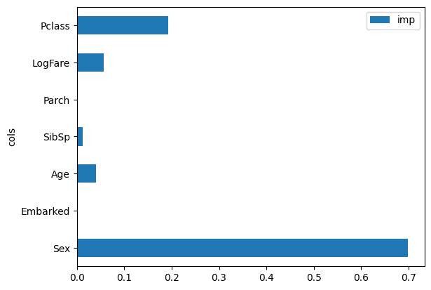
Random forests can tell us which independent variables were the most important in the model using feature importances.

# Feature Importance
pd.DataFrame(dict(cols=trn_xs.columns, imp=m.feature_importances_)).plot('cols', 'imp', 'barh')

<Axes: ylabel='cols'>

Paddy Doctor

Part 1

Load Data

creds = ''
dataFile = 'paddy-disease-classification'
path = loadData(creds, dataFile)

Downloading paddy-disease-classification.zip to /content

100%|██████████| 1.02G/1.02G [00:11<00:00, 94.5MB/s]

# check data files
! ls {path}

sample_submission.csv  test_images  train.csv  train_images

# set up default settings
from fastai.vision.all import *
set_seed(42)

path.ls()

(#4) [Path('paddy-disease-classification/sample_submission.csv'),Path('paddy-disease-classification/train_images'),Path('paddy-disease-classification/train.csv'),Path('paddy-disease-classification/test_images')]

Exploratory Data Analysis

trn_path = path/'train_images'
files = get_image_files(trn_path)

img = PILImage.create(files[0])
print(img.size)
img.to_thumb(128)

(480, 640)

# check image sizes in parallel
from fastcore.parallel import *

def f(o):
    return PILImage.create(o).size

sizes = parallel(f, files, n_workers=8)
pd.Series(sizes).value_counts()

(480, 640)    10403
(640, 480)        4
dtype: int64

Data Loaders

dls = ImageDataLoaders.from_folder(trn_path, valid_pct=0.2, seed=42,
    item_tfms=Resize(480, method='squish'),
    batch_tfms=aug_transforms(size=128, min_scale=0.75))

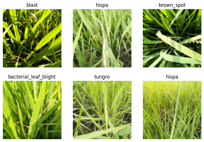
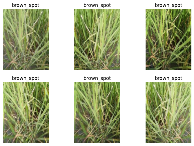
dls.show_batch(max_n=6)

First Model

learn = vision_learner(dls, 'resnet26d', metrics=error_rate, path='.').to_fp16()

Find Learning Rate

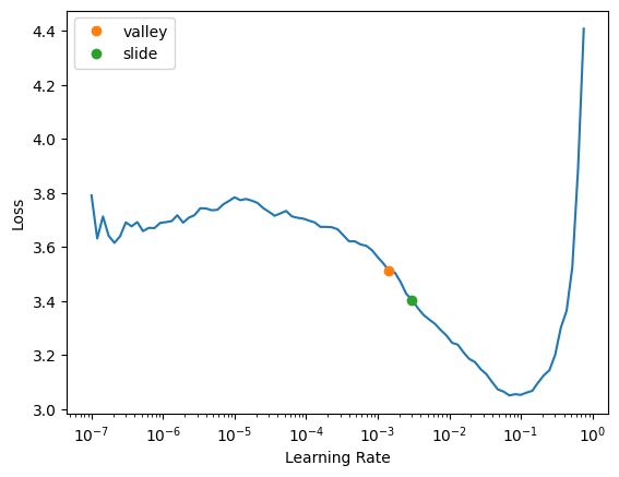
learn.lr_find(suggest_funcs=(valley, slide))

SuggestedLRs(valley=0.0014454397605732083, slide=0.0030199517495930195)

Train Model

learn.fine_tune(3, 0.01)

epoch	train_loss	valid_loss	error_rate	time
0	1.752005	1.081317	0.356079	01:20

epoch	train_loss	valid_loss	error_rate	time
0	1.155641	0.716448	0.227295	01:21
1	0.779499	0.463007	0.148967	01:21
2	0.545381	0.374054	0.116290	01:20

Submit to Kaggle

sample_sub = pd.read_csv(path/'sample_submission.csv')
sample_sub

	image_id	label
0	200001.jpg	NaN
1	200002.jpg	NaN
2	200003.jpg	NaN
3	200004.jpg	NaN
4	200005.jpg	NaN
...	...	...
3464	203465.jpg	NaN
3465	203466.jpg	NaN
3466	203467.jpg	NaN
3467	203468.jpg	NaN
3468	203469.jpg	NaN

3469 rows × 2 columns

# create test set
tst_files = get_image_files(path/'test_images').sorted()
tst_dl = dls.test_dl(tst_files)

# get model predictions for test set
probs,_,idxs = learn.get_preds(dl=tst_dl, with_decoded=True)
idxs

tensor([7, 8, 7,  ..., 8, 1, 5])

# map indexes to actual values
dls.vocab

['bacterial_leaf_blight', 'bacterial_leaf_streak', 'bacterial_panicle_blight', 'blast', 'brown_spot', 'dead_heart', 'downy_mildew', 'hispa', 'normal', 'tungro']

mapping = dict(enumerate(dls.vocab))
results = pd.Series(idxs.numpy(), name="idxs").map(mapping)
results

0                       hispa
1                      normal
2                       hispa
3                       blast
4                       blast
                ...          
3464               dead_heart
3465                    hispa
3466                   normal
3467    bacterial_leaf_streak
3468               dead_heart
Name: idxs, Length: 3469, dtype: object

## save submission
sample_sub['label'] = results
sample_sub.to_csv('part1_subm.csv', index=False)

!head part1_subm.csv

image_id,label
200001.jpg,hispa
200002.jpg,normal
200003.jpg,hispa
200004.jpg,blast
200005.jpg,blast
200006.jpg,brown_spot
200007.jpg,dead_heart
200008.jpg,brown_spot
200009.jpg,normal

Part 2

Load Data + Resize Images

trn_path = Path('sml')

# resize images to 192 x 256
resize_images(path/'train_images', dest=trn_path, max_size=256, recurse=True)

Data Loaders

dls = ImageDataLoaders.from_folder(trn_path, valid_pct=0.2, seed=42,
    item_tfms=Resize((256,192)))

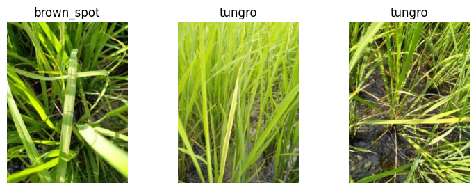
dls.show_batch(max_n=3)

Train Model

def train(arch, item, batch, epochs=5):
    dls = ImageDataLoaders.from_folder(trn_path, seed=42, valid_pct=0.2, item_tfms=item, batch_tfms=batch)
    learn = vision_learner(dls, arch, metrics=error_rate).to_fp16()
    learn.fine_tune(epochs, 0.01)
    return learn

Learner

learn = train('resnet26d', item=Resize(192),
              batch=aug_transforms(size=128, min_scale=0.75))

epoch	train_loss	valid_loss	error_rate	time
0	1.899457	1.388609	0.453628	00:26

epoch	train_loss	valid_loss	error_rate	time
0	1.295517	0.951328	0.316675	00:27
1	1.016938	0.664715	0.213359	00:28
2	0.712072	0.473869	0.157136	00:28
3	0.533225	0.334353	0.113407	00:27
4	0.444198	0.322105	0.107160	00:27

ConvNeXT Model

arch = 'convnext_small_in22k'

learn = train(arch, item=Resize(192, method='squish'),
              batch=aug_transforms(size=128, min_scale=0.75))

epoch	train_loss	valid_loss	error_rate	time
0	1.334298	0.838287	0.277271	00:33

epoch	train_loss	valid_loss	error_rate	time
0	0.660261	0.457503	0.147045	00:42
1	0.499239	0.358292	0.108602	00:41
2	0.326860	0.206613	0.064873	00:41
3	0.195506	0.147441	0.044210	00:42
4	0.122859	0.135444	0.043729	00:42

Preprocessing Experiments

Experiment 1: Square Cropping

learn = train(arch, item=Resize(192),
              batch=aug_transforms(size=128, min_scale=0.75))

epoch	train_loss	valid_loss	error_rate	time
0	1.322280	0.803323	0.258049	00:32

epoch	train_loss	valid_loss	error_rate	time
0	0.719919	0.449919	0.144642	00:39
1	0.554835	0.352141	0.111004	00:39
2	0.361483	0.254937	0.083133	00:39
3	0.213894	0.178465	0.053820	00:39
4	0.163988	0.167601	0.053820	00:39

Experiment 2: Padding

dls = ImageDataLoaders.from_folder(trn_path, valid_pct=0.2, seed=42,
                                   item_tfms=Resize(192, method=ResizeMethod.Pad, pad_mode=PadMode.Zeros))
dls.show_batch(max_n=3)

learn = train(arch, item=Resize((256,192), method=ResizeMethod.Pad, pad_mode=PadMode.Zeros),
              batch=aug_transforms(size=(171,128), min_scale=0.75))

epoch	train_loss	valid_loss	error_rate	time
0	1.268145	0.720653	0.234983	00:33

epoch	train_loss	valid_loss	error_rate	time
0	0.661217	0.485095	0.160980	00:43
1	0.548201	0.309334	0.091783	00:42
2	0.342416	0.222194	0.067756	00:55
3	0.213852	0.183673	0.053340	00:42
4	0.142283	0.149697	0.047093	00:45

Experiment 3: Time Test Augmentation

Test Time Augmentation - During the inference or validation, creating multiple versions of each image, using data augmentation, and then taking the average or maximum of the predictions for each augmented version of the image.

# check predictions and error rate of model without TTA
valid = learn.dls.valid
preds,targs = learn.get_preds(dl=valid)

# error (before TTA)
error_rate(preds, targs)

TensorBase(0.0471)

# data augmentation analysis
learn.dls.train.show_batch(max_n=6, unique=True)

# Time Test Augmentation
tta_preds,_ = learn.tta(dl=valid)

# error (after TTA)
error_rate(tta_preds, targs)

TensorBase(0.0404)

Scaling - Large Images + More Epochs

trn_path = path/'train_images'

learn = train(arch, epochs=12,
              item=Resize((480, 360), method=ResizeMethod.Pad, pad_mode=PadMode.Zeros),
              batch=aug_transforms(size=(256,192), min_scale=0.75))

epoch	train_loss	valid_loss	error_rate	time
0	1.092938	0.646208	0.207112	01:38

epoch	train_loss	valid_loss	error_rate	time
0	0.529627	0.281716	0.088419	01:45
1	0.395975	0.252327	0.083614	01:45
2	0.353087	0.355000	0.101874	01:44
3	0.296080	0.194901	0.058626	01:45
4	0.247156	0.180774	0.048534	01:45
5	0.188586	0.190078	0.045651	01:45
6	0.134304	0.152976	0.031235	01:45
7	0.110716	0.140041	0.030754	01:44
8	0.076065	0.121910	0.027871	01:46
9	0.056164	0.119214	0.026910	01:44
10	0.049165	0.114327	0.027391	01:45
11	0.035028	0.114869	0.027391	01:45

tta_preds,targs = learn.tta(dl=learn.dls.valid)
error_rate(tta_preds, targs)

TensorBase(0.0235)

Submit to Kaggle

tst_files = get_image_files(path/'test_images').sorted()
tst_dl = learn.dls.test_dl(tst_files)

# TTA for test set
preds,_ = learn.tta(dl=tst_dl)

# indices of largest prediction
idxs = preds.argmax(dim=1)

# find values in vocab
vocab = np.array(learn.dls.vocab)
results = pd.Series(vocab[idxs], name="idxs")

sample_sub = pd.read_csv(path/'sample_submission.csv')
sample_sub['label'] = results
sample_sub.to_csv('part2_subm.csv', index=False)
!head part2_subm.csv

image_id,label
200001.jpg,hispa
200002.jpg,normal
200003.jpg,blast
200004.jpg,blast
200005.jpg,blast
200006.jpg,brown_spot
200007.jpg,dead_heart
200008.jpg,brown_spot
200009.jpg,hispa

Acknowledgements

Summary

Jeremy Howard’s Advice

Load Data and Libraries

Exploratory Data Analysis

Exploratory Data Analysis: Data Preprocessing

Exploratory Data Analysis: Data Exploration

Binary Split

Simple Model - Categorical Variable Split: All females survive and no males do

Simple Model - Continuous Variable Split: Log Fare

Metric: Score Function

Decision Tree

Random Forests

Feature Importance

Paddy Doctor

Part 1

Load Data

Exploratory Data Analysis

Data Loaders

First Model

Find Learning Rate

Train Model

Submit to Kaggle

Part 2

Load Data + Resize Images

Data Loaders

Train Model

Learner

ConvNeXT Model

Preprocessing Experiments

Experiment 1: Square Cropping

Experiment 2: Padding

Experiment 3: Time Test Augmentation

Scaling - Large Images + More Epochs

Submit to Kaggle

Resources